Project Summary

Video Recap

Personal Objective

1. Apply recent AI learnings through a project-based format
2. Become familiar with the ML workflow (explore, develop, evaluate, select)
3. Get something up and running (and predicting 😂)

Exercise Objective

1. Develop a model to predict the hourly energy output of a power plant
2. Evaluate the performance of the model
3. Deploy the model for testing

Why Are These Predictions Important?

Accurately predicting how much energy a power plant can generate is crucial when planning out the supply and demand a city might need. If done incorrectly, inaccurate predictions could result in the rise of per-unit costs of electric power, power outages, and other unplanned difficulties.

Dataset

For this project, we'll be using the dataset CCPP from the  UCI Machine Learning repository (file attached below). The data was collected over the course of 6 years with 9,568 data points.

The columns in the data consist of hourly average ambient variables:

• Ambient Temperature (AT) in the range 1.81°C to 37.11°C,
• Ambient Pressure (AP) in the range 992.89-1033.30 millibar,
• Relative Humidity (RH) in the range 25.56% to 100.16%
• Exhaust Vacuum (V) in the range 25.36-81.56 cm Hg
• Net hourly electrical energy output (PE) 420.26-495.76 MW (Target we are trying to predict)

The Tooling

In this exercise, I used Google's VertexAI - a new low-code machine learning platform that makes it much easier for developers to deploy and maintain AI models.

Our Workflow

1. Exploratory Data Analysis
2. Develop the model
3. Evaluate the model
4. Select the best model

1. Exploratory Data Analysis

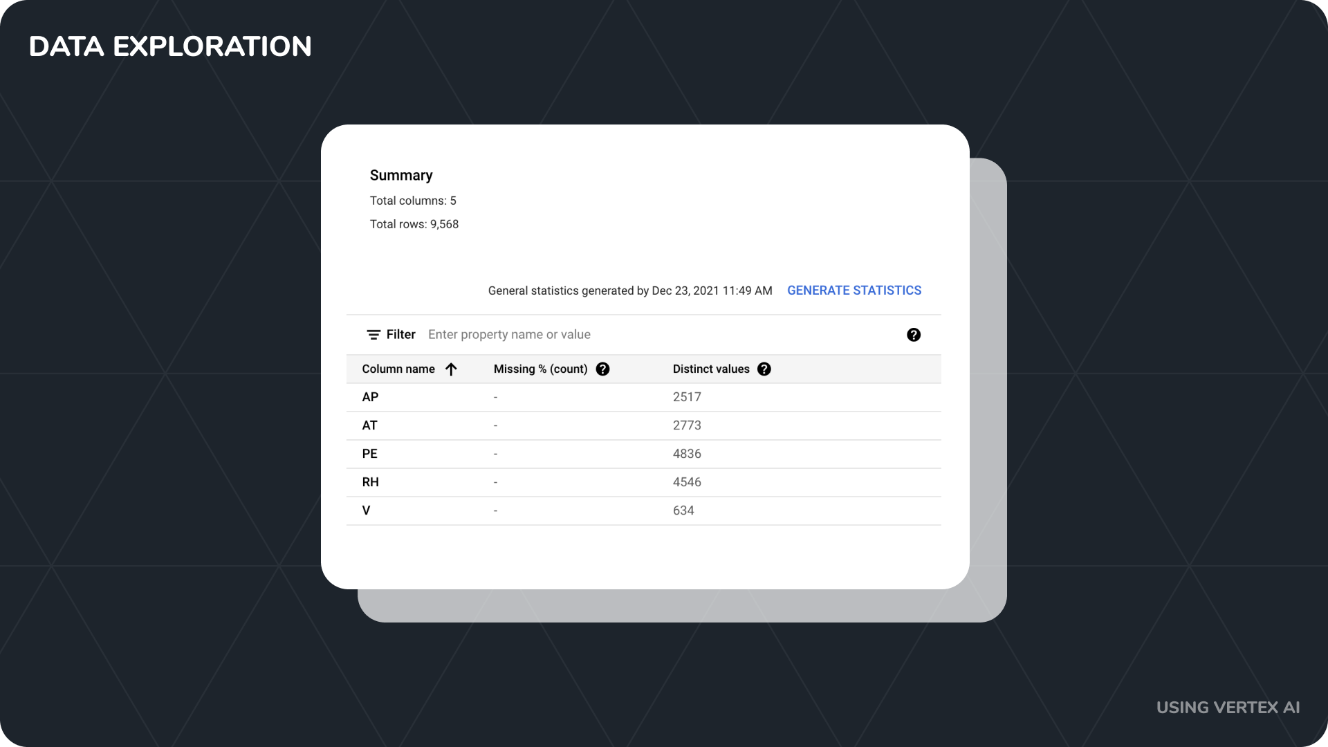
First, I took the CSV and uploaded it into Vertex AI for further exploration.

With over 9,000 rows, 5 numerical features, and no missing data the cleansing was quite straightforward.

After reviewing the data and getting familiar with it, I went ahead and started the model configuration.

2. Develop the Model

Since my dataset consists of numerical values and since we're looking to make a prediction - I knew some sort of regression model made the most sense.

Linear Regression

For this project, I chose  the linear regression algorithm for the reasons below:

• It's a simple model to configure and great for a "first stab"
• It's more interpretable/easier to understand when it comes to relationships between input (feature) and output (target) data
• Can be surprisingly effective

Model Training Configuration

VertexAI makes it a breeze when it comes to selecting a model and configuring the training options.

Once I had my training set up, it was time to select the target outputs that I wanted to predict.

Selecting the Target Feature and Splitting the Training and Test Data

Since Net hourly electrical energy output is what we're trying to predict, I chose PE as our Target Column.

Also, a nice thing about Google's VertexAI is that it does the training & test data splitting for you (see image above)!

I did this a few times with several different models and configurations and found a strong correlation between one of the input features.

Evaluating the Feature Correlation and Importance

I came to discover that Ambiant Temperature AT  is one of the most important features when it comes to correlation to our target output!

Weighting Our Correlated and Important Feature

With that, I decided to weight the AT column more than the other model feature inputs.

And in order to measure the model errors appropriately with an effort to penalize large errors, in particular, I chose to go with Root Mean Squared Error RMSE.

3. Evaluate the Model

Once the model was done training I evaluated the model error metrics.

Evaluate the Model Error Metrics

Mean absolute error (MAE) is the average of absolute differences between observed and predicted values. A low value indicates a higher-quality model, where 0 means the model made no errors. Interpreting MAE depends on the range of values in the series. MAE has the same unit as the target column.

The mean absolute percentage error (MAPE) is the average of absolute percentage errors. MAPE ranges from 0% to 100%, where a lower value indicates a higher quality model. MAPE becomes infinity if 0 values are present in the ground truth data.

Root mean square error (RMSE) is the root of squared differences between observed and predicted values. A lower value indicates a higher-quality model, where 0 means the model made no errors. Interpreting RMSE depends on the range of values in the series. RMSE is more responsive to large errors than MAE.

Root mean squared log error (RMSLE) is the root of squared averages of log differences between observed and predicted values. Interpreting RMSLE depends on the range of values in the series. RMSLE is less responsive to outliers than RMSE, and it tends to penalize underestimations slightly more than overestimations.

r squared (r^2) is the square of the Pearson correlation coefficient between the observed and predicted values. This ranges from 0 to 1, where a higher value indicates a higher-quality model.

Great, so with a lower RMSE, I went ahead and began building the endpoint for model deployment 🚀

4. Deploying Our Model

Once the endpoint was named, I entered the model settings (traffic split, compute nodes, and machine type) and hit deploy!

So simple.

...  about 10 minutes later the model was ready to go for a spin!

Testing with Test Data

Using our test data I entered a few inputs into V , AP, and RH to generate predictions 🥁...  

... and voila, we had a prediction (see outputs above in yellow) in a matter of seconds!

Let's walk through this.

Our Predictions

Our first example (1st row below "predictions") stated that:

• with an Exhaust Vacuum (V) of 62.96
• and Ambient Pressure (AP) of 1020.04
• and  Relative Humidity (RH) of 59.08

... 🥁

This lands our model ~95% prediction interval with an RMSE of 4.841.

Now at a first glance, this seems great, however, my gut tells me this is most likely overfitted... but nonetheless I've made my first prediction!

Wrap Up

With a model that is most likely overfitted, my next step would be to try different regression algorithms like Decision Tree Regression and Random Forest Regression for example, until we've evaluated all of our options to find out which one returned the best performance.

However, since I only had a weekend to work on this project this was all the time I had and as a whole, I hit all of my project and personal objectives!

What I Learned

1. First-hand experience developing a linear regression model
2. Better understanding to how the UX might assist in training models more efficiently
3. The importance of feature correlation and weighting

I hope you found this quick blog insightful and, at the very least, saw that approaching numerical problems with artificial intelligence doesn't have to be rocket science or overcomplicated!

Until next time!